Comparative Genomics: How to Compare Bacterial and Microbial Genomes

Comparative genomics asks what makes genomes similar and different — how closely two organisms are related, which genes they share, and what distinguishes one strain or species from another. For bacteria and other microbes, where genomes are compact but gene content varies enormously between strains, these comparisons drive taxonomy, outbreak investigation, and our understanding of how traits like resistance and virulence spread. This guide covers the core methods, from single-number similarity metrics to genome-wide gene-content and structural comparisons.

The scale of microbial genomics has transformed what comparative analysis can do. Sequencing has become cheap enough that studies routinely involve dozens, hundreds, or thousands of genomes, and public databases hold vast collections of reference sequences to compare against. This has shifted the field from examining single genomes in isolation to thinking about whole populations — how diversity is structured within a species, how genes flow between strains, and where the boundaries between species actually lie. The workflow reflects that breadth: it moves from single-number similarity metrics that place an organism taxonomically, through gene-content analysis that explains functional differences, to structural comparison and finally an evolutionary framework. No single tool answers every question, so comparative genomics is best understood as a coordinated set of methods, each suited to a particular aspect of how genomes are alike and how they differ.

What comparative genomics answers

At its core, comparative genomics answers a few linked questions: Are these two genomes the same species? How closely related are these strains? Which genes do they share, and which are unique? and How is their gene order arranged? Different tools address different questions, and a complete study usually combines several — a similarity metric to place organisms taxonomically, gene-content analysis to explain phenotypic differences, and alignment to reveal structural changes.

Step 1 — Prerequisites

Comparative genomics is only as reliable as its inputs. That means quality-checked assemblies (fragmented or contaminated genomes distort every comparison) and consistent annotation across all genomes, so that genes are called the same way in each. Using assemblies of very different quality, or annotations from different tools and versions, introduces differences that are technical artefacts rather than biology. Standardising these up front — the groundwork covered in our bacterial WGS guide — is what makes the comparisons meaningful.

Step 2 — Average nucleotide identity (ANI)

ANI is the standard way to express how genetically similar two genomes are in a single number: the mean nucleotide identity across the regions they share. Its power lies in a well-established threshold — genomes of the same species typically share ~95% ANI or higher (a value that corresponds closely to the older 70% DNA–DNA hybridisation standard), while different species fall well below it. FastANI computes this rapidly using alignment-free approximate mapping, making all-versus-all comparisons of many genomes practical; alignment-based variants (ANIb using BLAST, ANIm using MUMmer) also exist. ANI is the go-to tool for confirming species identity and for de-replicating redundant genomes in large datasets. Alongside the ANI value, the alignment fraction — how much of the two genomes actually aligns — is worth reporting, because high identity over only a small shared region means something quite different from high identity across most of both genomes.

Step 3 — Orthology and gene content

To compare what genomes do, you compare their genes. Orthologues are genes in different genomes descended from a common ancestral gene, and identifying them is the basis of gene-content comparison. Tools such as OrthoFinder group genes across genomes into orthogroups, revealing which genes are universally shared and which are present in only some genomes. This distinction — shared “core” genes versus variable “accessory” genes — is what explains many phenotypic differences between otherwise similar strains.

Step 4 — Pan-genome analysis

Scaling gene-content comparison across many isolates of a species yields the pan-genome: the full set of genes found across the group. Tools such as Roary and Panaroo partition genes into the core genome (present in essentially all isolates) and the accessory genome (soft-core, shell, and cloud categories by how widely shared they are). The core genome provides a stable backbone for phylogenetics, while the accessory genome — enriched for mobile elements, resistance, and virulence genes — captures the variable content that often distinguishes strains and explains outbreaks.

Step 5 — Whole-genome alignment and synteny

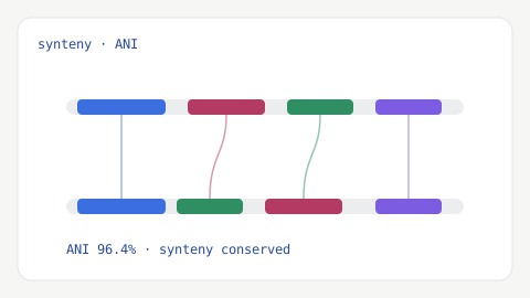
Beyond gene presence, comparative genomics examines gene order. Whole-genome alignment with tools such as MUMmer (nucmer), minimap2, or Mauve reveals synteny — conserved blocks of gene order between genomes — and, by contrast, the structural rearrangements (inversions, translocations, insertions, and deletions) that distinguish them. Synteny analysis is informative because closely related genomes usually preserve gene order, so breaks in synteny point to genuine evolutionary events, mobile-element activity, or, sometimes, assembly artefacts worth double-checking.

Step 6 — Phylogenomics

Comparative genomics and phylogenetics come together in phylogenomics: building an evolutionary tree from genome-scale data, typically a core-genome alignment derived from the pan-genome analysis. This places all the compared genomes into an explicit evolutionary framework, turning pairwise similarities into a picture of how the whole set is related. The alignment, model-selection, and support considerations are the same as in any rigorous tree-building exercise — covered in our phylogenetics guide.

Applications

These methods underpin much of modern microbiology. Taxonomy uses ANI to define and assign species. Outbreak and surveillance work uses core-genome comparison to determine how closely isolates are related. Functional and evolutionary studies use pan-genome and orthology analysis to track the gain and loss of resistance, virulence, and metabolic genes — connecting genotype to phenotype across a population. Together they turn a collection of genomes into an understanding of a species’ diversity and history, which is central to our infectious-disease work.

Common pitfalls

The recurring comparative-genomics mistakes are avoidable. Comparing assemblies of very different quality confounds biology with technical noise. Inconsistent annotation makes shared genes look different across genomes. Reading too much into a single ANI value near a boundary ignores the alignment fraction and biological context. Mistaking assembly errors for rearrangements in synteny analysis invents evolution that isn’t there. And relying on one gene rather than genome-scale data gives a partial picture. Standardised inputs and documented methods — the way we run every comparison — keep the conclusions sound.

Detecting selection and functional change

Comparative genomics can go beyond cataloguing gene presence to ask how genes are evolving. A central tool is the dN/dS ratio (also written ω or Ka/Ks) — the ratio of non-synonymous (amino-acid-changing) to synonymous (silent) substitutions in a protein-coding gene. A ratio near 1 suggests neutral evolution, well below 1 indicates purifying selection preserving the protein, and above 1 points to positive selection driving change. Frameworks such as PAML (codeml) and HyPhy estimate these, helping identify genes under adaptive pressure — often those involved in host interaction, immune evasion, or antibiotic resistance.

Comparison also extends to function. Once orthogroups and accessory genes are identified, functional annotation (against databases like KEGG, GO, or COG) and enrichment analysis reveal which kinds of functions differ between groups of genomes — for example, whether a lineage has gained metabolic capabilities or lost them. This shifts the analysis from “these genomes differ” to “they differ in these biologically meaningful ways,” which is usually the conclusion that matters. As always, statistical care is needed so that enrichment reflects real signal rather than annotation bias.

Conclusion

Comparing microbial genomes well means using the right tool for each question — ANI for relatedness and species boundaries, orthology and pan-genome analysis for gene content, whole-genome alignment for synteny, and phylogenomics to tie it together — all built on quality assemblies and consistent annotation. Done carefully, comparative genomics turns a set of sequences into real insight about a species. If you’d like your genomes compared and interpreted rigorously, our team handles the full workflow — tell us what you’re comparing.

Frequently asked questions