RNA-seq Analysis: A Complete Guide from FASTQ to Differential Expression

RNA sequencing has become the default way to ask which genes change between two biological conditions — a treatment versus a control, a tumour versus adjacent tissue, a knockout versus wild type. The wet-lab part ends when the sequencer writes out a set of FASTQ files. Everything that determines whether your conclusions are trustworthy happens afterwards, in the analysis. This guide walks the full RNA-seq workflow from raw reads to a defensible list of differentially expressed genes, and flags the decisions that quietly make or break a result.

What RNA-seq actually measures

RNA-seq counts sequencing reads that originate from transcribed RNA. After library preparation, each gene or transcript is represented by a number of reads roughly proportional to its abundance in the sample — but only roughly, because that number also depends on transcript length, library size, GC content, and the composition of the rest of the sample. The entire computational pipeline exists to convert those raw, biased counts into a fair comparison between conditions. Keeping that goal in mind explains why each step below is necessary rather than ceremonial.

A crucial design point comes before any code runs: biological replication. Three replicates per condition is a practical minimum; more is better. Sequencing one sample very deeply cannot substitute for replicates, because depth reduces technical noise but tells you nothing about biological variability — and it is biological variability that a differential expression test must estimate to separate real change from chance.

Step 1 — Quality control of raw reads

Start by looking at the data. FastQC summarises per-base quality, adapter content, duplication, and GC distribution for each FASTQ file, and MultiQC aggregates those reports across an entire experiment so outlier samples stand out immediately. Typical issues include residual adapter sequence, a drop in quality toward read ends, and over-representation of a few sequences.

Where trimming is needed, tools such as fastp or Trimmomatic remove adapters and low-quality tails. A word of caution: aggressive trimming can do more harm than good. Modern splice-aware aligners soft-clip poor read ends anyway, so heavy quality trimming often removes usable signal without improving results. The right amount of trimming is the minimum that fixes a real problem you can see in the QC report.

Step 2 — Alignment vs. pseudo-alignment

There are two mainstream routes from reads to per-gene numbers. The first is genome alignment with a splice-aware aligner such as STAR or HISAT2, which place each read on the reference genome, correctly spanning exon–exon junctions. The second is transcript-level quantification with Salmon or kallisto, which skip base-to-base alignment and instead assign reads to transcripts probabilistically — far faster and lighter on memory.

For a standard gene-level differential expression study, pseudo-alignment is an excellent default: it is quick, accurate, and handles reads that map to multiple isoforms gracefully. Choose genome alignment when you need the aligned reads themselves — for novel transcript discovery, variant calling from RNA, or visualising coverage in a genome browser. Whichever route you take, use a well-curated annotation such as GENCODE or Ensembl, and keep the genome and annotation versions consistent across every sample and documented in your methods.

Step 3 — Quantification

Quantification turns placements into a matrix of genes (rows) by samples (columns), where each cell is a count. Two unit systems appear constantly and are easy to confuse. Counts are integer read tallies and are the correct input to differential expression tools. TPM (transcripts per million) is a within-sample normalised unit useful for comparing the relative abundance of genes inside one sample, but it is not appropriate as the input to a count-based statistical test. A common mistake is to feed TPM or FPKM into a tool expecting raw counts; keep counts for statistics and reserve TPM for visualisation and quick relative comparisons.

When using Salmon, the tximport package imports transcript estimates and summarises them to gene level while carrying across an offset that corrects for average transcript length — the statistically correct way to move from transcripts to genes.

Step 4 — Normalisation

You cannot compare raw counts between samples directly. If one library was sequenced twice as deeply, every gene in it will show roughly twice the counts — a purely technical difference. Subtler still is composition bias: if a handful of genes dominate one condition, they consume reads that would otherwise have been distributed across other genes, deflating everything else.

The standard tools handle this with well-established methods. DESeq2 uses a median-of-ratios size factor, while edgeR uses TMM normalisation; both estimate a per-sample scaling factor that accounts for depth and composition. This is one of the most important steps in the pipeline and one of the least visible — get it wrong and every downstream comparison inherits the error. Our biostatistics team treats normalisation and the modelling that follows as the analytical heart of an RNA-seq project.

Step 5 — Differential expression

With a normalised count matrix and a clear experimental design, differential expression testing asks, for each gene, whether the change between conditions is larger than expected given the noise. Count data are modelled with a negative binomial distribution, which captures the over-dispersion typical of RNA-seq — variance that grows faster than the mean. DESeq2, edgeR, and limma-voom are the three workhorses; in practice they agree closely on well-designed experiments.

Two ideas make these tools reliable on small sample sizes. First, information sharing: dispersion is estimated across all genes and shrunk toward a trend, so a gene with three replicates borrows strength from thousands of others. Second, fold-change shrinkage: log2 fold-change estimates for low-count genes are pulled toward zero, preventing the huge, meaningless ratios that noisy low-expression genes would otherwise produce. Specify your design formula deliberately — if samples were processed in batches, include the batch term (~ batch + condition) so the model separates the effect you care about from the nuisance you don’t.

Step 6 — Interpretation and enrichment

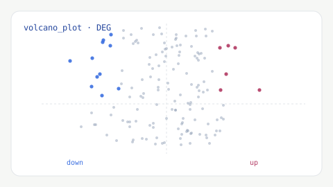
The output is a table with, per gene, a log2 fold change, a p-value, and an adjusted p-value. Because you tested tens of thousands of genes, you must control the false discovery rate; the Benjamini–Hochberg adjusted p-value (often called the FDR or q-value) does this. Filter on the adjusted value — typically below 0.05 — not the raw p-value. Pair that statistical threshold with a fold-change threshold so your hit list is both significant and biologically meaningful, and visualise the result with a volcano plot (significance versus fold change) and an MA plot (fold change versus mean expression).

A gene list is rarely the endpoint. Functional enrichment asks what those genes have in common: over-representation analysis tests whether particular Gene Ontology terms or pathways appear more than expected, while GSEA uses the entire ranked list and avoids arbitrary cutoffs. This is where a differential expression result becomes a biological story — and where publication-ready figures and methods take shape.

Common pitfalls

A handful of mistakes account for most unreliable RNA-seq results. Too few replicates is the most common: with two per group there is almost no power to estimate variability. Unmodelled batch effects are the most dangerous — if all treated samples were processed on one day and controls on another, you cannot tell biology from batch unless the design accounts for it. Others include feeding TPM into a count-based test, filtering on raw rather than adjusted p-values, and changing genome or annotation versions midway through a project. Each is avoidable with a documented, reproducible pipeline — which is exactly why we wrap RNA-seq workflows into versioned, re-runnable pipelines.

Making the pipeline reproducible

A result that cannot be reproduced is a liability, not an asset — and reviewers increasingly ask for the evidence. The practical answer is to treat the whole RNA-seq workflow as software. Wrap each tool in a container (Docker or Singularity) so the exact version is fixed, and orchestrate the steps with a workflow manager such as Nextflow or Snakemake rather than a hand-run list of commands. Community pipelines like nf-core/rnaseq bundle QC, trimming, quantification, and reporting into a single tested, versioned workflow that runs the same way on a laptop, a cluster, or the cloud.

Two habits pay for themselves many times over. First, pin every version — genome build, annotation release, and each tool — and record them in the output, so “we used GENCODE v44 and Salmon 1.10” is a fact you can point to rather than a memory. Second, keep a single aggregated MultiQC report per project as a living quality dashboard; when a sample misbehaves months later, that report explains why. These practices are what let a methods section be written precisely, a collaborator re-run your analysis, and a result still hold up a year on — and they are the backbone of every pipeline we build.

Conclusion

RNA-seq is conceptually simple — count reads, compare conditions — but each step hides a decision that shapes the final list. Quality control catches problems early; the alignment or pseudo-alignment choice trades speed for flexibility; quantification must preserve counts for statistics; normalisation makes samples comparable; and a well-specified model with FDR control turns noise-aware statistics into biology you can defend to a reviewer. Get those right and the result reproduces. If you’d like this handled end to end on your data, our transcriptomics service covers the full path from FASTQ to figures.

Frequently asked questions