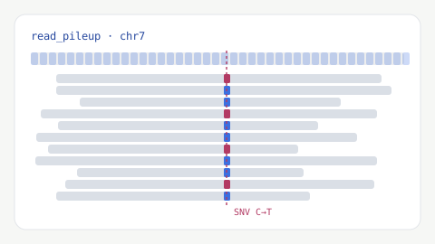
A variant call file (VCF) looks deceptively simple: a list of positions where a sample differs from the reference genome. Producing one you can trust is anything but simple. Between the raw reads and that final list sits a sequence of steps — each correcting a specific source of error — codified by the Broad Institute as the GATK best-practices workflow. This guide walks that pipeline from aligned reads to an annotated, filtered VCF, and explains why each step exists, because understanding the reasoning is what lets you spot when something has gone wrong. It underpins our genomics and variant analysis service.
Key takeaways
- Every step in the pipeline corrects a specific, known source of error — none is optional decoration.
- Joint genotyping across samples produces better calls than genotyping each sample alone.
- Raw calls must be filtered; an unfiltered VCF is full of false positives.
- Germline and somatic calling are different problems and use different tools.
From reads to variants: the big picture
The goal is to distinguish true genetic differences from the many artefacts that sequencing introduces: alignment errors near indels, optical and PCR duplicates that fake confidence, systematic miscalibration of quality scores, and sequencing noise that mimics rare variants. The best-practices workflow is a pipeline of corrections applied in a deliberate order, ending in a statistical model that separates real variants from noise. Skipping steps does not just lose a little accuracy — it lets specific, predictable classes of false positive through.
Step 1 — Alignment
Everything begins by placing reads on the reference genome. For short reads, BWA-MEM is the long-standing standard, producing a BAM file of aligned reads. Two details matter downstream. First, assign correct read groups — metadata identifying sample, library, and sequencing lane — because later steps model error at the read-group level. Second, use the exact reference build your project standardises on (for example GRCh38) and keep it consistent everywhere; mixing builds is a silent, costly error.
Step 2 — Mark duplicates
PCR amplification and optical effects create duplicate reads — multiple copies of the same original fragment. If left in, they inflate apparent read depth and make a variant look better supported than it really is. Picard MarkDuplicates (also built into GATK) flags these so the caller counts each original fragment once. The reads are marked rather than deleted, preserving the raw data while preventing duplicates from biasing the call.
Step 3 — Base Quality Score Recalibration
Every base carries a quality score estimating the probability it was read incorrectly, but sequencers make systematic errors — scores drift with machine cycle, sequence context, and other covariates. Base Quality Score Recalibration (BQSR) builds an empirical model of these patterns using known variant sites (from resources like dbSNP) as truth, then adjusts the scores so they reflect true error rates. Because the variant caller weighs evidence by base quality, well-calibrated scores directly improve call accuracy. This is one of the least glamorous and most quietly important steps in the pipeline.
Step 4 — Calling with HaplotypeCaller
With clean, recalibrated reads, GATK HaplotypeCaller identifies variants. Rather than inspecting one base at a time, it locally reassembles reads into candidate haplotypes in active regions — places that look variable — which makes it far more accurate around indels, where naive position-by-position callers stumble. Run per sample, it emits a GVCF: a genomic VCF that records evidence at every position, including confidence that a site is reference, not just where variants were found. That extra information is what makes the next step possible.
Step 5 — Joint genotyping
When you have several samples, genotyping them together rather than separately produces materially better calls. Joint genotyping combines the per-sample GVCFs and calls across the whole cohort at once, which sharpens genotype assignment at low-coverage sites and distinguishes a true homozygous-reference call from missing data. It also yields a consistent, square set of sites across all samples — essential for any downstream population or association analysis. The GVCF-then-joint-genotyping design also scales: adding a new sample does not require re-calling the entire cohort from scratch.
Step 6 — Filtering
Raw calls are not final calls. An unfiltered VCF contains many false positives, and the job of filtering is to flag them while keeping true variants. GATK offers two routes. Variant Quality Score Recalibration (VQSR) trains a model on known true and false sites to score each call — powerful, but it needs many variants and good truth resources, so it suits whole-genome cohorts. Hard filtering applies threshold rules on annotations such as quality-by-depth, strand bias, and mapping quality, and is the pragmatic choice for single samples or small panels where VQSR lacks enough data. SNVs and indels are filtered separately because they have different error profiles. Whichever route, filtering is not optional: shipping an unfiltered VCF as a result is one of the most common mistakes we see.
Step 7 — Annotation
A filtered VCF tells you where variants are; annotation tells you what they might mean. Tools such as Ensembl’s VEP or SnpEff predict each variant’s effect — which gene and transcript it hits, whether it changes a protein, and its likely consequence. Population frequency from gnomAD helps triage: a variant common in the general population is unlikely to cause a rare disease. For clinical context, ClinVar links variants to reported significance. Interpreting these responsibly — separating a plausible candidate from a confirmed cause — is the substance of variant interpretation, and we treat predictions as hypotheses that need validation, never as diagnoses.
SNVs, indels, and structural variants
The workflow above excels at single-nucleotide variants (SNVs) and short insertions and deletions (indels). Larger events — copy-number changes, large deletions, inversions, and translocations, collectively structural variants — need different tools that reason over read pairs, split reads, and depth, and long-read sequencing resolves many of them far better than short reads. If your biological question involves large rearrangements, a short-read SNV pipeline alone will miss them; the method has to match the variant class you care about.
Germline vs. somatic calling
Germline calling assumes clean genotypes — roughly 0%, 50%, or 100% variant allele fraction — inherited in every cell. Somatic calling, as in cancer, is a different problem: tumours are mixtures of subclones and normal cells, so variants appear at arbitrary, often low allele fractions, and must be separated from germline background and sequencing noise. GATK Mutect2 is built for this, typically comparing tumour to a matched normal and a panel of normals. Using a germline caller on tumour data — or vice versa — produces misleading results, which is why our oncology and oncogenomics work keeps the two pipelines distinct.
Common pitfalls
Most unreliable VCFs trace to a short list of errors. Shipping unfiltered calls tops it — the raw output is not a result. Mixing reference builds between alignment, recalibration, and annotation silently corrupts coordinates. Skipping duplicate marking or BQSR lets predictable artefacts through. Genotyping samples separately when they should be called jointly weakens low-coverage calls. And using the wrong caller for germline versus somatic data invalidates the analysis outright. Every one is avoidable with a documented, versioned pipeline — the same reproducibility we build into every custom pipeline, so a reviewer or collaborator can re-run the analysis and reach the same VCF.
Validating your VCF
Once you have a filtered, annotated VCF, the last question is whether to trust it — and there are objective ways to check. A few whole-callset metrics act as a quick health check. The transition/transversion (Ti/Tv) ratio should sit near expected values for your capture (around 2.0–2.1 for whole genomes, higher for exomes); a ratio far from that signals excess false positives. The number of variants and the ratio of known (in dbSNP) to novel calls should match expectations for the sample type and ancestry.
For rigorous validation, benchmark against a truth set. The Genome in a Bottle (GIAB) reference samples come with high-confidence variant calls, and tools such as hap.py compare your VCF to that truth within defined confidence regions, reporting precision and recall for SNVs and indels separately. In family studies, checking Mendelian consistency in trios — a child’s genotypes should be explicable by the parents’ — catches errors that per-sample metrics miss. Adequate, even coverage underpins all of it: thin or uneven coverage produces unreliable genotypes no downstream step can fix. Building these checks into the pipeline turns “the calls look fine” into a measured, reportable statement of quality — the standard we hold every variant analysis to.
Conclusion
Variant calling is a chain of corrections, each addressing a specific error, ending in a statistical decision about what is real. Align carefully, mark duplicates, recalibrate, call into GVCFs, genotype jointly, filter deliberately, and annotate with population and clinical context — and you get a VCF you can defend. Cut a corner and you inherit a predictable class of false positive. If you’d like this run end to end on your WGS or WES data, with every tool and reference version documented, our variant analysis service takes it from FASTQ to an interpreted, filtered VCF.