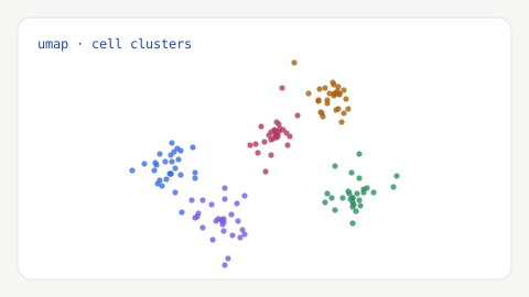
Single-cell RNA sequencing measures gene expression one cell at a time, resolving the cell-type composition of a tissue and the states within each population — detail that bulk RNA-seq averages away. That power comes with a longer, more decision-heavy analysis than bulk work, where quality-control and clustering choices directly shape the biological conclusions. This guide walks the full scRNA-seq workflow from raw reads to annotated cell types, following the current community best practices.
Key takeaways
- Quality control choices propagate: they affect normalisation, which affects clustering, which affects interpretation.
- QC thresholds should be derived from your own data’s distributions, not copied as fixed cutoffs.
- Doublets and ambient RNA are real artefacts with dedicated correction tools — don’t skip them.
- Clusters are not cell types until annotated; UMAP is for visualisation, not for measuring distances.
What scRNA-seq measures
Most current experiments use droplet-based platforms (such as 10x Genomics Chromium), which encapsulate individual cells with barcoded beads. Each transcript carries a cell barcode (identifying its droplet) and a unique molecular identifier, or UMI (tagging the original molecule so PCR duplicates can be collapsed). The output of primary processing is a large, sparse gene-by-cell count matrix. Understanding that structure — barcodes, UMIs, and pervasive zeros — explains why the downstream steps look different from bulk RNA-seq.
Step 1 — From reads to a count matrix
Primary processing demultiplexes cell barcodes, collapses UMIs, and aligns or maps reads to the transcriptome to produce the count matrix. 10x Genomics’ Cell Ranger is the standard for its platform; STARsolo and alevin-fry are fast, open alternatives that produce equivalent matrices. This step also makes an initial call about which barcodes correspond to real cells versus empty droplets containing only ambient RNA.
Step 2 — Quality control
QC removes technical artefacts so that each remaining observation is, as far as possible, one intact cell. Three covariates do most of the work: the total UMI count (count depth), the number of detected genes, and the fraction of mitochondrial reads. Cells with low counts and few genes but a high mitochondrial fraction typically have broken membranes — dying cells whose cytoplasmic mRNA has leaked out, leaving mostly mitochondrial transcripts. Cells with unusually high counts and gene numbers are often doublets (two cells in one droplet).
Two points matter here. First, thresholds should come from your data: a mitochondrial cutoff that is strict for one tissue is permissive for another, so inspect the distributions and set data-specific thresholds rather than copying a fixed recipe. Second, two artefacts deserve dedicated tools. Doublets can be flagged with Scrublet, scDblFinder, or DoubletFinder, which simulate artificial doublets and score each barcode against them. Ambient RNA — the background “soup” of cell-free transcripts from lysed cells — can be estimated and subtracted with SoupX or CellBender. Skipping these steps leaves contamination that can create spurious clusters or blur real ones.
Step 3 — Normalisation and feature selection
Raw counts differ between cells largely because of capture and sequencing depth, so they must be normalised before comparison. The common approach is depth normalisation followed by a log transform; model-based alternatives such as SCTransform are also widely used. You then select highly variable genes — the few thousand genes that carry most of the biological signal — to focus the downstream analysis and reduce noise from uninformative genes.
Step 4 — Dimensionality reduction
Even after feature selection, the data have thousands of dimensions. Principal component analysis (PCA) compresses the highly variable genes into a smaller set of components that capture the dominant axes of variation. A nearest-neighbour graph is then built in this PCA space, which becomes the basis for both clustering and visualisation. Choosing how many principal components to keep is a real decision that affects the structure you recover.
Step 5 — Batch integration
When a study spans multiple samples, runs, or donors, technical batch effects can dominate biological signal — cells may cluster by sample rather than by type. Integration methods align shared cell populations across batches while aiming to preserve genuine biological differences; Harmony, scVI, and Seurat’s CCA-based integration are common choices. Integration is powerful but not free: over-correction can erase real biology, so it should be applied deliberately and its effect checked, which is exactly the kind of judgement our biostatistics team brings to single-cell work.
Step 6 — Clustering
Cells are grouped by community detection on the nearest-neighbour graph. The Leiden algorithm is the current standard (an improvement on the older Louvain), and its resolution parameter controls how finely the data are split. There is no single correct resolution: raising it produces more, smaller clusters and lowering it produces fewer, broader ones. The right setting depends on the biological question, and it is normal to try several and evaluate them — clustering is an exploratory step, not a fixed answer.
Step 7 — Visualisation
UMAP (and, historically, t-SNE) projects the high-dimensional data to two dimensions for visualisation. These embeddings are invaluable for seeing structure, but they come with an important caveat: distances and cluster sizes in a UMAP are not quantitatively meaningful. Two clusters sitting far apart on a UMAP are not necessarily more different than two that sit close, and the visual should never be used to infer relationships that the underlying data don’t support. Treat it as a map, not a measurement.
Step 8 — Marker genes and cell-type annotation
Clusters are just groups of similar cells until you assign identities. For each cluster you compute differentially expressed marker genes — those it expresses more than the rest — and compare them against known canonical markers for the tissue (for example, established markers for T cells, B cells, monocytes, and so on). Reference-based automated annotation tools can speed this up by comparing your cells to labelled reference atlases, but their calls should always be checked against markers and biological plausibility. This is where careful, honest annotation matters most: it is tempting to over-interpret a small cluster, and the disciplined answer is sometimes “an intermediate or ambiguous state” rather than a confident label. Robust cell-type identification underpins downstream analyses such as differential abundance and trajectory inference across our immunology and oncology work.
Common pitfalls
The recurring single-cell mistakes are methodological, not computational. Copying fixed QC thresholds across tissues removes real cells or keeps bad ones. Skipping doublet and ambient-RNA handling leaves artefacts that masquerade as biology. Reading distances off a UMAP invents relationships. Over-clustering and then labelling noise as rare cell types produces confident-looking but unsupported claims. And ignoring batch effects lets technical structure drive the clustering. Each is avoidable with a reproducible, well-documented pipeline — the standard we hold every workflow to.
Beyond clustering: downstream analyses
Annotated cell types are a foundation, not an endpoint. Several downstream analyses turn them into biological answers, and each has its own methodological care. Differential abundance asks whether the proportion of a cell type changes between conditions — treated versus control, for example — which requires accounting for the compositional nature of the data and for the number of replicates. Differential expression between conditions within a cell type is best done with a pseudobulk approach (aggregating counts per sample per cell type and using established bulk methods), because treating individual cells as independent replicates dramatically inflates false positives — a well-documented pitfall.
Two further analyses are common. Trajectory inference (with tools such as Monocle, Slingshot, or PAGA) orders cells along inferred developmental or activation paths, useful when a process is continuous rather than discrete — though inferred trajectories are hypotheses that need validation, not established lineages. Cell–cell communication analysis (with CellPhoneDB or CellChat) infers signalling between cell types from ligand–receptor expression. All of these amplify whatever happened upstream, so their reliability rests on sound QC, integration, and annotation.
Experimental design considerations
No amount of analysis rescues an underpowered single-cell experiment, and the most consequential decisions are made before sequencing. Cell number determines whether rare populations are captured at all — detecting a cell type present at 1% reliably requires capturing enough cells that it appears in meaningful numbers. Sequencing depth per cell (reads per cell) trades off against the number of cells for a fixed budget; the right balance depends on whether the goal is broad cell-type discovery (favouring more cells) or fine transcriptional detail (favouring more depth).
The single most common design flaw is confusing cells with replicates. For any comparison between conditions, biological replicates — independent samples or donors per group — are what allow generalisable conclusions; thousands of cells from one animal are not a substitute for several animals, because they share that individual’s biological and technical idiosyncrasies. Where samples must be pooled to save cost, multiplexing approaches such as cell hashing or genetic demultiplexing let multiple samples share a run while remaining separable, which also helps control batch effects. Designing for adequate cells, depth, and true replication is what makes the downstream statistics meaningful.
Conclusion
Single-cell RNA-seq is a chain of linked decisions: quality control shapes normalisation, normalisation shapes clustering, and clustering shapes the cell types you report. Done carefully — data-specific QC, honest artefact handling, deliberate integration, and annotation checked against biology — it delivers a resolved, defensible picture of a tissue. If you’d like this run end to end on your data, our transcriptomics service covers single-cell analysis from raw reads to annotated, publication-ready results.