Whole Exome Sequencing (WES) Analysis: From FASTQ to Variant Interpretation

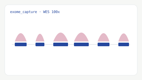
The exome — the ~1–2% of the genome that codes for proteins — harbours the large majority of currently interpretable disease-causing variants. Whole exome sequencing (WES) targets that fraction, which makes it cheaper than whole-genome sequencing and lets you sequence it much more deeply for the same budget. This guide walks the full WES workflow from raw FASTQ files to classified, interpretable variants, and highlights the capture-specific steps that distinguish it from WGS.

What WES is, and when to use it

WES uses hybridisation capture to enrich the coding exons before sequencing. Commercial capture kits — Agilent SureSelect, Twist Bioscience, and IDT xGen among them — differ in exactly which regions they target and how evenly they capture them, which is why the capture kit is part of your methods, not a detail. Because only a small fraction of the genome is sequenced, you can reach high depth affordably: this is the core appeal of WES for Mendelian-disease gene discovery and coding-variant studies. The flip side is that capture is never perfectly uniform, so coverage varies across targets in a way that WGS does not.

Step 1 — Quality control

As with any sequencing project, start with FastQC and MultiQC to review per-base quality, adapter content, and duplication. WES libraries often show higher duplication than WGS because of the enrichment step, so duplication levels are worth watching. Trim adapters if the QC report shows real contamination, but avoid aggressive quality trimming that removes usable read ends.

Step 2 — Alignment

Reads are aligned to the reference genome (GRCh38 for current human work) with BWA-MEM. Assign correct read groups, and — as always — keep the reference build identical across every sample and every downstream step. The whole exome is aligned against the whole genome; the restriction to target regions comes later, so off-target reads are handled rather than discarded at this stage.

Step 3 — Duplicate marking and recalibration

Duplicates are marked with Picard/GATK MarkDuplicates, and base qualities are recalibrated with BQSR, exactly as in the GATK best-practices workflow. Duplicate marking is especially important for WES because the enrichment and PCR steps raise duplication rates, and uncorrected duplicates would inflate apparent support for variants.

Step 4 — On-target metrics

Here is the step that has no WGS equivalent. Using the capture kit’s target BED file, you compute enrichment and coverage metrics: the fraction of reads that fall on target, the mean target depth, and — critically — the percentage of target bases covered at useful thresholds (for example, at ≥20×). These numbers define what your assay can and cannot see. A gene that falls in a poorly captured, GC-rich, or repetitive region may be effectively invisible even in a high-mean-depth exome, so per-target coverage, not just the overall average, is what determines sensitivity.

Step 5 — Variant calling

Small variants are called with a haplotype-aware caller — GATK HaplotypeCaller (emitting GVCFs for joint genotyping across a cohort) or DeepVariant. Calling is typically restricted to the target regions (with a small padding, since capture pulls in flanking bases). Joint genotyping across multiple exomes improves genotype accuracy at lower-coverage sites and yields a consistent set of positions across all samples.

Step 6 — Coverage and quality metrics

Clinical-grade WES commonly targets a mean depth of around 100×, with roughly 95% of target bases covered at ≥20× to reliably call both homozygous and heterozygous genotypes; published ACMG laboratory guidance describes similar coverage expectations. Note that real-world exomes frequently cover only about 90–95% of targets at ≥20×, so a fraction of exonic bases is under-covered in every run. Exome data also has a characteristic Ti/Tv ratio of roughly 3.0–3.3 — higher than the ~2.0–2.1 of whole genomes, because coding regions are enriched for transitions — and a value far from that range is a useful red flag.

Step 7 — Annotation

Annotation turns coordinates into candidate biology. Ensembl VEP or SnpEff predict transcript consequences; population frequency from gnomAD separates common from rare; and ClinVar supplies previously reported clinical assertions. Aggregated predictor sets (such as dbNSFP) and specialised tools — SpliceAI for splicing effects, and computational missense predictors — add supporting evidence. These predictions inform, but do not by themselves establish, pathogenicity.

Step 8 — ACMG/AMP variant classification

Clinical interpretation follows the ACMG/AMP 2015 framework (Richards et al.), which weighs multiple lines of evidence into a five-tier classification: Pathogenic, Likely Pathogenic, Uncertain Significance (VUS), Likely Benign, and Benign. Evidence criteria carry different strengths — for example, a predicted loss-of-function variant in a gene where loss of function causes disease is very strong pathogenic evidence, while an allele frequency far too high for the disorder is stand-alone benign evidence. Tools such as InterVar help automate the initial criteria assignment, and computational predictors can contribute supporting evidence, but they are not sufficient on their own; final classification requires expert review. The honest, and clinically standard, outcome is that many variants land in the VUS category — interesting but not actionable without further evidence. Handling that ambiguity carefully is the substance of variant interpretation.

Limitations of exome sequencing

WES is powerful but bounded. It sees coding regions and near-splice-site bases, so it misses deep intronic and regulatory variants that WGS would capture. Capture is uneven, so some exons are chronically under-covered. And copy-number and structural variant detection is harder and less reliable from exome data than from WGS, because CNV inference from capture data must contend with target-to-target coverage variability. When non-coding variation or robust structural analysis is central to the question, WGS is the better instrument — a trade-off worth deciding before sequencing, not after.

Common pitfalls

The recurring WES mistakes are specific: reporting mean depth without per-target coverage, which hides blind spots; ignoring the capture kit’s target regions during calling and QC; treating a VUS as a finding; expecting reliable CNVs from a design that is not built for them; and the universal one, mixing reference builds across steps. A documented, versioned pipeline — the kind we build for every project — prevents most of these, and makes the analysis reproducible for a reviewer or collaborator.

Trio and family-based analysis

For rare-disease diagnosis, sequencing an affected individual together with their parents — a trio — substantially improves interpretation, and it is one of the most effective ways to raise diagnostic yield. The reason is that a trio lets you determine each variant’s inheritance pattern directly. De novo variants — present in the child but neither parent — are strong candidates for dominant disorders, and they can only be identified confidently when both parents are sequenced. Recessive models become testable too: you can confirm that two variants in the same gene are on different chromosomes (in trans, one from each parent), as compound heterozygosity requires.

Trios also improve data quality. Checking Mendelian consistency — whether a child’s genotypes are explicable by the parents’ — flags genotyping errors that per-sample metrics miss, and genotype-refinement approaches use the pedigree to improve calls. The practical effect is a much shorter, better-prioritised candidate list: instead of thousands of rare variants, inheritance filtering focuses attention on the handful consistent with the disease model, which is why trio designs are standard in clinical exome analysis.

Secondary and incidental findings

Because WES sequences all protein-coding genes, it can reveal medically important variants unrelated to the reason for testing — for example a pathogenic variant in a cancer-predisposition or cardiac gene found while investigating an unrelated condition. The American College of Medical Genetics and Genomics maintains a defined list of genes (updated periodically) for which it recommends reporting such secondary findings in clinical exome and genome sequencing, because they are considered medically actionable — the associated conditions can be prevented or treated if identified.

This raises analytical and ethical considerations that belong in the study design, not as an afterthought. Analytically, the secondary-findings genes must be well covered and carefully interpreted even though they are not the primary target. Ethically, whether and how to return such findings involves patient consent and the right not to know, which is why clinical workflows handle them under explicit policies. For research WES, the same capability means teams should decide in advance how incidental medically relevant findings will be handled, rather than confronting the question only when one appears.

Conclusion

WES is a cost-effective, high-depth view of the protein-coding genome, and it remains the workhorse for coding-variant and Mendelian-disease studies. Its distinctive steps — capture-aware on-target metrics, coverage reporting at the per-target level, and ACMG-guided classification — are what turn an exome dataset into a defensible interpretation. If you’d like this handled end to end, from FASTQ to classified variants and a publication-ready write-up, our genomics and variant analysis service covers the full path.

Frequently asked questions