Whole-genome sequencing reads essentially every base of an organism’s DNA — coding and non-coding alike — which makes it the most complete view of genetic variation available today. The trade-off is that a WGS dataset is large, and turning billions of short reads into a variant list a biologist can act on takes a disciplined, reproducible pipeline. This guide walks the full WGS workflow from raw FASTQ files to an interpretable set of variants, and explains why each step exists.
Key takeaways
- WGS gives near-uniform coverage across coding and non-coding regions, without the capture bias of targeted assays.
- Around 30× average depth is the accepted standard for confident germline variant calling.
- WGS resolves structural and copy-number variants that exome and panel sequencing largely miss.
- Every variant is a hypothesis: annotation and interpretation, not the caller, decide what matters.
What WGS captures
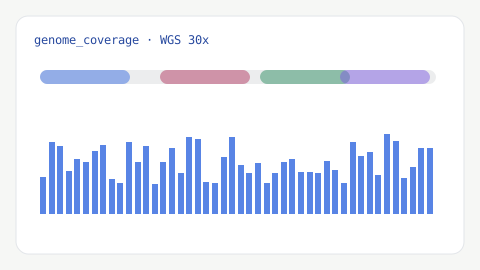
Unlike exome or panel sequencing, WGS does not enrich for specific regions, so coverage is comparatively even across the genome. That uniformity matters: it lets you detect variants in promoters, introns, intergenic regions, and regulatory elements, and it makes copy-number and structural analysis far more reliable because there are no capture-induced coverage gaps. For a human germline sample, an average depth of about 30× is the widely used standard — enough to call heterozygous and homozygous genotypes confidently across most of the genome. Somatic (tumour) applications need considerably more depth to detect low-frequency variants.
Step 1 — Read quality control
Begin by inspecting the raw reads with FastQC and aggregating across samples with MultiQC. You are checking per-base quality, adapter content, duplication levels, and GC distribution. Light adapter and quality trimming (with fastp or Trimmomatic) is sometimes warranted, but modern aligners soft-clip poor read ends anyway, so heavy trimming often removes usable signal without improving calls. The goal is to catch real problems — a failed lane, heavy adapter contamination — not to over-process.
Step 2 — Alignment
Reads are aligned to a reference genome — for human work, GRCh38 is the current standard build. BWA-MEM (and the faster BWA-MEM2) is the long-established aligner; hardware-accelerated platforms such as Illumina DRAGEN are common in high-throughput settings. Two practices matter here: assign correct read-group metadata (sample, library, lane), because downstream error models work at that level, and keep the reference build consistent across every sample and every later step. Mixing genome builds silently corrupts coordinates and is one of the costliest mistakes in a genomics project.
Step 3 — Duplicate marking and recalibration
PCR and optical duplicates inflate apparent depth and make a variant look better supported than it is, so they are flagged (not deleted) with Picard/GATK MarkDuplicates. Base Quality Score Recalibration (BQSR) then corrects systematic biases in the per-base quality scores using known variant sites as truth. Because the variant caller weighs evidence by base quality, well-calibrated scores translate directly into more accurate calls. These steps follow the widely adopted GATK best-practices framework.
Step 4 — Small-variant calling (SNVs and indels)
Single-nucleotide variants and short insertions/deletions are called with a haplotype-aware caller. GATK HaplotypeCaller locally reassembles reads into candidate haplotypes, which improves accuracy around indels, and emits a per-sample GVCF that records confidence at every position. Google’s DeepVariant, a deep-learning caller, is another strong option that performs very well on WGS. When you have a cohort, joint genotyping across all GVCFs produces better calls than genotyping samples separately — it sharpens low-coverage genotypes and yields a consistent set of sites across every sample, which is essential for downstream population analysis.
Step 5 — Structural and copy-number variants
This is where WGS earns its cost. Structural variants (SVs) — large deletions, duplications, inversions, and translocations — and copy-number variants (CNVs) are poorly captured by exome and panel assays because those methods have uneven, targeted coverage. WGS’s even coverage makes them tractable. Dedicated callers reason over read pairs, split reads, and read depth: Manta, DELLY, and GRIDSS are widely used for SVs, while tools such as CNVnator and cn.MOPS handle copy number. Short reads still struggle with SVs in repetitive regions; long-read sequencing resolves many of these far better, so the sequencing technology should match the variant classes you care about.
Step 6 — Filtering and annotation
Raw calls are not final calls. Small variants are filtered with GATK VQSR (for large cohorts with good truth resources) or hard filters (for single samples), with SNVs and indels handled separately because they have different error profiles. Annotation then turns coordinates into meaning: Ensembl VEP or SnpEff predict each variant’s consequence, population frequency from gnomAD helps triage common from rare, and ClinVar links variants to reported clinical significance. Interpreting these responsibly — distinguishing a plausible candidate from a confirmed cause — is the substance of variant interpretation.
Coverage and quality metrics
A few whole-callset metrics tell you quickly whether to trust the output. Mean depth should sit near your target (about 30× for germline), with a high fraction of the genome above ~20×. The transition/transversion (Ti/Tv) ratio should be around 2.0–2.1 for whole genomes; a value far from that signals excess false positives. Mapping rate, duplication rate, and the ratio of known-to-novel variants are also worth checking. These sanity checks take minutes and catch problems that would otherwise propagate into the biology.
From variants to biological insight
A raw callset can contain four to five million variants for a human genome, so the interpretive work is prioritisation: filtering by consequence, frequency, inheritance model, and biological plausibility to reach a short list worth pursuing. Throughout, the honest framing is that a called and annotated variant is a hypothesis, not a conclusion — predicted effects and pathogenicity scores need experimental or clinical validation before they carry weight. That discipline is what separates a defensible result from an over-interpreted one, and it is central to how we approach genomics projects.
Common pitfalls
A handful of mistakes account for most unreliable WGS results. Insufficient depth undermines genotype confidence. Mixing reference builds between alignment, recalibration, and annotation corrupts coordinates silently. Shipping unfiltered calls presents raw output as a result. Ignoring structural variants wastes one of WGS’s main advantages. And relying on short reads in repetitive regions misses variants a long-read approach would resolve. Each is avoidable with a documented, versioned pipeline — the reproducibility we build into every custom pipeline.
Germline versus somatic WGS
The workflow above assumes germline analysis, where variants are inherited and present in essentially every cell at clean genotype frequencies (~0%, 50%, or 100%). Somatic WGS — as in cancer — is a different problem. A tumour sample is a mixture of tumour and normal cells and of tumour subclones, so somatic variants appear at arbitrary, often low variant-allele fractions and must be separated from germline background and sequencing noise. This requires dedicated somatic callers such as GATK Mutect2 or Strelka2, ideally comparing the tumour to a matched normal sample from the same individual, plus a panel of normals to filter recurrent artefacts.
Two tumour-specific factors shape the analysis. Tumour purity (the fraction of tumour cells in the sample) and ploidy directly affect the observed allele fractions, so they must be estimated to interpret variants correctly, and low-purity samples need greater depth to detect real mutations. Subclonal architecture means some variants are present in only a fraction of tumour cells, which is biologically informative but analytically demanding. Using a germline caller on tumour data — or vice versa — produces misleading results, so the two pipelines are kept distinct from the outset.
Reference genomes: GRCh38 and beyond
Every alignment-based result is expressed relative to a reference genome, so the choice of reference is a scientific decision, not a technicality. For human work, GRCh38 is the current standard and remains the reference of record for clinical and most research analysis. It improved substantially on GRCh37/hg19 — better representation of segmental duplications and the addition of alternate haplotypes — which is why coordinates and results are not interchangeable between builds.
More recently, the Telomere-to-Telomere (T2T) Consortium produced T2T-CHM13, the first truly complete human genome assembly, filling in centromeres, segmental duplications, and other regions that were gaps or placeholders in GRCh38. It resolves variants in previously inaccessible regions and is increasingly used in research, though clinical pipelines have been slower to migrate because databases, annotations, and validation are built around GRCh38. The practical guidance is to pick one build deliberately, use it consistently across alignment, recalibration, and annotation, and record it explicitly in your methods — and to be cautious when comparing results generated against different references.
Conclusion
WGS is the most complete view of a genome, but that completeness only becomes useful through a careful pipeline: quality control, consistent alignment, best-practice processing, haplotype-aware small-variant calling, dedicated structural and copy-number analysis, and disciplined filtering, annotation, and interpretation. Get those right and the result reproduces and holds up to scrutiny. If you’d like this handled end to end on your data, our genomics and variant analysis service takes it from FASTQ to an interpreted callset.